What is VLOOKUP?

VLOOKUP, short for Vertical Lookup is an Excel function that lets you join data from different tables or find data that is in a different table based on a search criteria and returns the first matched value. VLOOKUP simplifies tasks like finding corresponding information.

Understanding how to leverage the function can significantly enhance your ability to navigate and make sense of complex datasets.

Syntax: VLOOKUP(lookup_value, table_array, col_index_num, [range_lookup])

In the simplest form, this is how VLOOKUP works: "Look for this value (look_up value) in this data range (table array) and when you find it, return the corresponding value in column number(col_index_number), optional(Exact match(0) or the closest match less or equal to the lookup value(1)"

Before we dive into what the arguments mean, you have to understand the following terms first.

Lookup table: The table that has data or information that you need to be retrieve based on the search criteria.

Source table: The table where you have the value that you want to use as the lookup criteria. This value is used to search the lookup table and find the related information

Now lets figure out what the arguments mean.

Lookup_value : The value in the source table that you are looking for in the lookup table.

Table_array: The data range of the lookup table which has data you want to search through. It should include the column with the lookup_value as the leftmost column and the column from which you want to retrieve the result. It should be written in the absolute form. To quickly transform your range into absolute form after selecting it click F4.

Col_index_num : The number of the column in the lookup table you want to be returned after a match is found, relative to the range you defined in the table array.

Range_lookup : An optional argument that determines whether you want an approximate match or an exact match. Use TRUE or 1 for an approximate match (find the closest value less than or equal to the lookup_value), and use FALSE or 0 for an exact match. If not specified, excel uses approximate match as default which sometimes gives unexpected results.

The best way to get it is by practicing. Excel shows the formula description when you type it in, for reference.

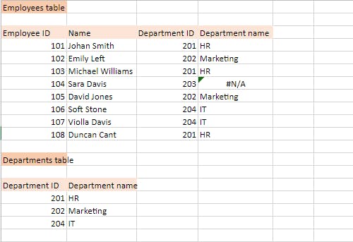
Let's look at an example use of VLOOKUP in the Employees table to retrieve the department name from the Department table, provided the Department ID.

After getting the first value, drag the formula down to the rest of the cells. Remember if you don't make the range absolute you will get errors. Below is our final output.

Important to note:

If an exact match is not found and range_lookup is set to FALSE, VLOOKUP will return the #N/A error.

The best way to handle it is to use another function IFERROR to catch the error.

Syntax =IFERROR(VLOOKUP(lookup_value, table_array, col_index_num, [range_lookup]), value_if_error)

IFERROR takes two arguments.

The action to be taken, in this case our VLOOKUP function, and the alternative action to be taken if an error occurs.

Case example using our tables:

Department ID 203 has been removed, our function does not find the match in the Departments table. It gives an error as shown below.

To fix this, you should edit your existing vlookup function as follows;

=IFERROR(VLOOKUP(C4, $A$16:$B$18, 2, FALSE),"Not Found")